Exam 2 Practice

These are practice problems for the exam to help you review the main concepts covered since the last exam. Please also be sure to review homework problems, readings, and class notes.

Problems

• Open Intro Statistics [OI]: 3.13, 3.18, 3.32

• Open Intro Statistics [OI]: 4.4 , 4.6

• Introduction to Modern Statistics [IMS]: 13.5

Additional Problems

For questions 1 we will consider the speed_gender_height data from the openintro package. This data set contains the recordings of 1,292 UCLA students. These students were asked to fill out a survey where they were asked about their height, fastest speed they have ever driven, and gender. Here are the first ten rows of data.

speed_gender_height |> head(10)

# A tibble: 10 × 3
   speed gender height
   <int> <fct>   <dbl>
 1    85 female     69
 2    40 male       71
 3    87 female     64
 4   110 female     60
 5   110 male       70
 6   120 female     61
 7    90 female     65
 8    90 female     65
 9    80 female     61
10    95 male       69

Question 1

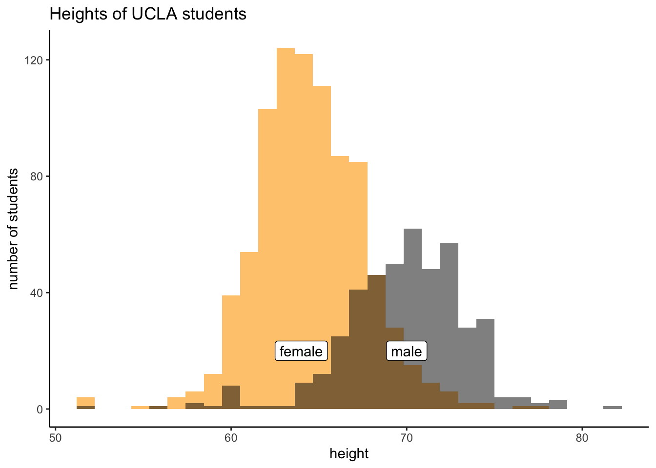
1. Consider the histogram of heights of male and female participants from a UCLA survey below created with the raw data. Do the two distributions represent data distributions, sampling distributions, or bootstrap distributions?

Solution

They are both data distributions.

2. Does it seem like a normal distribution would be a good fit for these distributions?

Solution

And they are roughly normal.

3. Consider the summary statistics below. Assuming the two groups are normally distributed, write the shorthand notation for distribution for each of the male and female heights of students from this survey.

gender	Mean	Std.Dev	n
female	64.35	2.99	863
male	69.64	3.54	439

Solution

Let X be female heights

Let Y be male heights

\(X \sim N(64.35, 2.99)\)

\(Y \sim N(69.64, 3.54)\)

4. Calculate a 95% confidence interval for the mean of each group.

Solution

\(\bar{X}\sim N(64.35, \frac{2.99}{ \sqrt{863}})\)

\(\bar{Y} \sim N(69.64, \frac{3.54}{\sqrt{439}})\)

The observe that \(\sigma_\overline{x} = \frac{2.99}{ \sqrt{863}}\approx 0.1018\). We can calculate our confidence bounds using the following formulas,

The 95% confidence interval for female heights is thus \[[64.15, 64.55].\]

The observe that \(\sigma_\overline{y} = \frac{3.54}{\sqrt{439}} \approx 0.1690\). We can calculate our confidence bounds using the following formulas,

The 95% confidence interval for male heights is thus \[[69.31, 69.97].\]

5. You will not be able to bootstrap on the exam, but you can still consider the bootstrap distribution. Suppose all female-identifying UCLA students are the population, and recall our sample has 863 female-identifying students in it. If you were to guess, what would your bootstrap distribution look like for mean hieght of female-identifying students? Write the notation.

Solution

The bootstrap distribution is an approximation of the sampling distribution. Knowing nothing else one would guess it is centered around \(\overline{x}\) with a standard error very close to the sampling distribution.

\(\overline{X}_{boot}\sim N(64.35, \frac{2.99}{ \sqrt{863}})\)

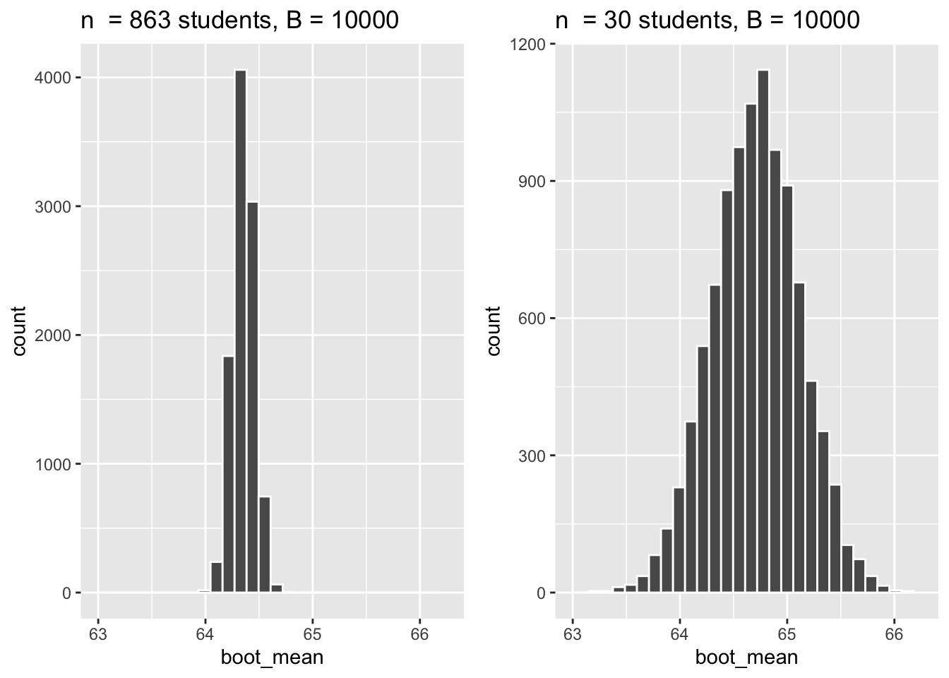
6. Consider two subsets of the speed_gender_height data. The first subset contains all 863 female-identifying students from the original data set. The second subset only contains the 30 female-identifying students from the original data set. Two bootstrap distributions (\(B = 10,000\)) were created from these data sets and are plotted below. How do the distributions differ?

Solution

• Center: The bootstrap distribution is typically centered around the mean of the data set that was used to generate the distribution. So for the \(n = 863\) data set we would typically expect the center to be around the sample mean we calculated earlier, \(\overline{x} = 64.35\). For the smaller data set \(n = 30\) the sample mean could be something different. Since it is generally coming from the same source we do not expect it to be that different, but it could be. The sample is smaller so a mean estimated with only 30 observations could be erratic.

• Spread: The bootstrap distribution approximates the sampling distribution. Since both samples have \(n \geq 30\) we do expect the sampling distribution to be approximately normal. However, the standard error is equal to \(SE = \frac{\sigma_x}{\sqrt{n}} = \frac{2.99}{\sqrt{n}}\). From this formula we can see that the standard error (or spread of the sampling distribution) gets smaller as \(n\) increases. This is what we observe for the two bootstrap distributions above.

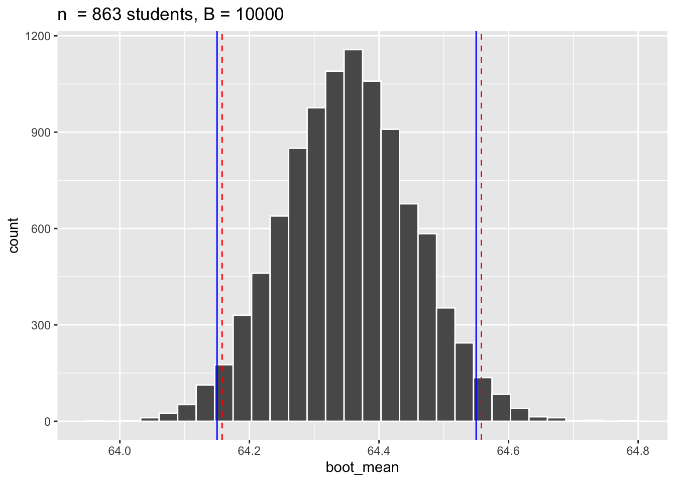
7. If we calculated a 95% bootstrap confidence interval of heights using the \(n = 863\) female-identifying students how would it compare to the confidence interval we generated in question 1c?

Solution

The bootstrap confidence interval is in red, and the confidence in question 3 is in blue. We can see that these intervals are incredibly similar, as they both are created based on an approximation of the sampling distribution using data.

8. If we make a 99% bootstrapped confidence interval how will that compare to the bootstrap confidence interval in question 1g?

Solution

It’ll be wider. We are more confident that we have captured the true value.

1. Interpret your confidence interval for female-identifying students created in 1c.

Solution

We are 95% confident that the confidence interval [64.15, 64.55] captures the true mean (\(\mu\)) height of female-identifying students at UCLA.

10. A friend claims that female-identifying students at UCLA have an average height of 70 inches. Write out the null and alternative hypotheses that correspond to this claim. Using a 95% confidence interval, would you believe your friend’s claim?

Solution

\(H_o: \mu=70\)

\(H_a: \mu \ne 70\)

This height is many standard errors outside our confidence interval, if we trust our sample is representative of female-identifying UCLA students we should not believe such nonsense and conclude the null hypothesis is likely false.

Question 2

In a recent study 109 moderately obese subjects were given a low-carbohydrate diet. The prediction was that the subjects would lose weight on the average. After two years, the mean change was -5.5 kg with a standard deviation of 7.0 kg.

1. What population is under consideration in the data set?

Solution

The moderately obese adults.

2. What parameter is being estimated?

Solution

The mean (\(\mu\)) weight in kilograms lost over 2 years on a low-carbohydrate diet.

3. What is the point estimate for the parameter?

Solution

We estimate the mean using \(\overline{x}\).

4. What is the name of the statistic we use to measure the uncertainty of the point estimate?

Solution

Standard error (SE) is the standard deviation of \(\overline{x}\).

5. Compute the value from part 2d for this context.

Solution

Standard error (SE) is estimated using \(\sigma_\overline{x} = \frac{\sigma_x}{\sqrt{n}} = \frac{7}{\sqrt{109}} \approx 0.67\).

6. A recent magazine claimed that following a low-carbohydrate diet can help people lose 2 kg per week. How would you set up your hypothesis to test if the claimed rate agrees with the data observed from the study?

Solution

We need to change the claim of the magazine to be in 2yrs, instead of 1 week. This way it matches the data we collected. Assuming the rate is the same, the claim of the magazine would change to \(H_0: \mu = 208\), and \(H_A: \mu \neq 208\).