library(tidyverse)
library(palmerpenguins)
library(broom)
library(infer)
library(kableExtra)

penguins <- na.omit(penguins)Penguin Themed Exam 3 Review
To prepare for Exam 3, be sure to review homework problems, readings, and class notes. In addition, below are some practice problems we have highlighted in particular.
Previous/Book Problems
IMS Problems: 25.4, 25.8
Additional Problems
Packages
Consider the penguins data from palmerpenguins package in R. This data set includes measurements for various penguins in the island Palmer Archipelago. For simplicity, we removed the rows with NA values.
Problem 1
The table below contains a summary of statistics for the body_mass_g variable for each species. Find a 95% confidence interval for the body mass of the Gentoo. Be sure to mention any relevant conditions. If you use R, only consider the functions: pt(), qt(), pnorm(), qnorm().
penguins |>
  group_by(species) |>
  summarize(n = n(),
            sd = sd(body_mass_g),
            min = min(body_mass_g),
            max = max(body_mass_g),
            mean = mean(body_mass_g),
            median = median(body_mass_g))
# A tibble: 3 × 7
species n sd min max mean median
<fct> <int> <dbl> <int> <int> <dbl> <dbl>
1 Adelie 146 459. 2850 4775 3706. 3700
2 Chinstrap 68 384. 2700 4800 3733. 3700
3 Gentoo 119 501. 3950 6300 5092. 5050Problem 2
Describe and contrast each of the following. Be as specific as you can. You can use the penguins data set as an example if you would like.
A Data Distribution
A Randomization Distribution
A Sampling Distribution
Problem 3
Suppose we wanted to test if mean body mass of the three types of penguins is the same.
Write the appropriate null and alternative hypotheses for this test. For each, write the hypothesis both in words (as one complete sentence) and using a mathematical statement involving population parameters.
What conditions should I consider?
Which conditions can be relaxed and how?
The R output for this test is provided below. Fill in the three ? below (without using R).
results <- aov(body_mass_g ~ species, data = penguins)
tidy(results)| term | df | sumsq | meansq | statistic | p.value |
|---|---|---|---|---|---|
| species | ? | 146864214 | 73432107.1 | ? | 2.892368e-82 |
| Residuals | ? | 72443483 | 213697.6 | NA | NA |
Problem 4
Test the hypothesis that the proportion of female penguins on Biscoe is 50%. Check conditions. Do as much of this by hand/calculator as you can. If you use R, only consider the functions: pt(), qt(), pnorm(), qnorm().
filter(.data = penguins, island == "Biscoe") |>
count(island, sex)
# A tibble: 2 × 3
island sex n
<fct> <fct> <int>
1 Biscoe female 80
2 Biscoe male 83Problem 5
Consider the following R output.
| term | estimate | std.error | statistic | p.value |
|---|---|---|---|---|
| (Intercept) | 17.229501 | 3.2818483 | 5.249938 | 6.595397e-07 |
| bill_depth_mm | 2.020768 | 0.2185866 | ? | 1.015502e-15 |
What are the conditions for a linear regression using a mathematical model (like the one above)? Do we know if the data meet those conditions? Explain.
Fill in the blanks: The R output displays a linear model for the Gentoo penguins where the __________ variable is
bill_depth_mmand the __________ variable isbill_length_mm.Without computing the model yourself find the value for ? above.
Make a 90% confidence interval for the slope of the regression equation. If you use R, only consider the functions:
pt(), qt(), pnorm(), qnorm().In plain english interpret the slope 2.02 and intercept 17.23 from the output above.
Solution
a. Conditions:
Our data need be linear. (see graph)
Our data need to be independent and we assume it is.
The residuals should be roughly normal. (see residual graph)
The variability of our data should be relatively constant. (see graph)
Without using R it is tricky to check all of these conditions. Below is a point plot and a plot of the residuals to show that they are met. There is one outlier, but its not too far out…
penguins_gentoo <- filter(penguins, species == "Gentoo")
penguins_gentoo |>
  ggplot(aes(x=bill_length_mm, y= bill_depth_mm))+
  geom_point() +
  geom_smooth(method = "lm", se= FALSE)
`geom_smooth()` using formula = 'y ~ x'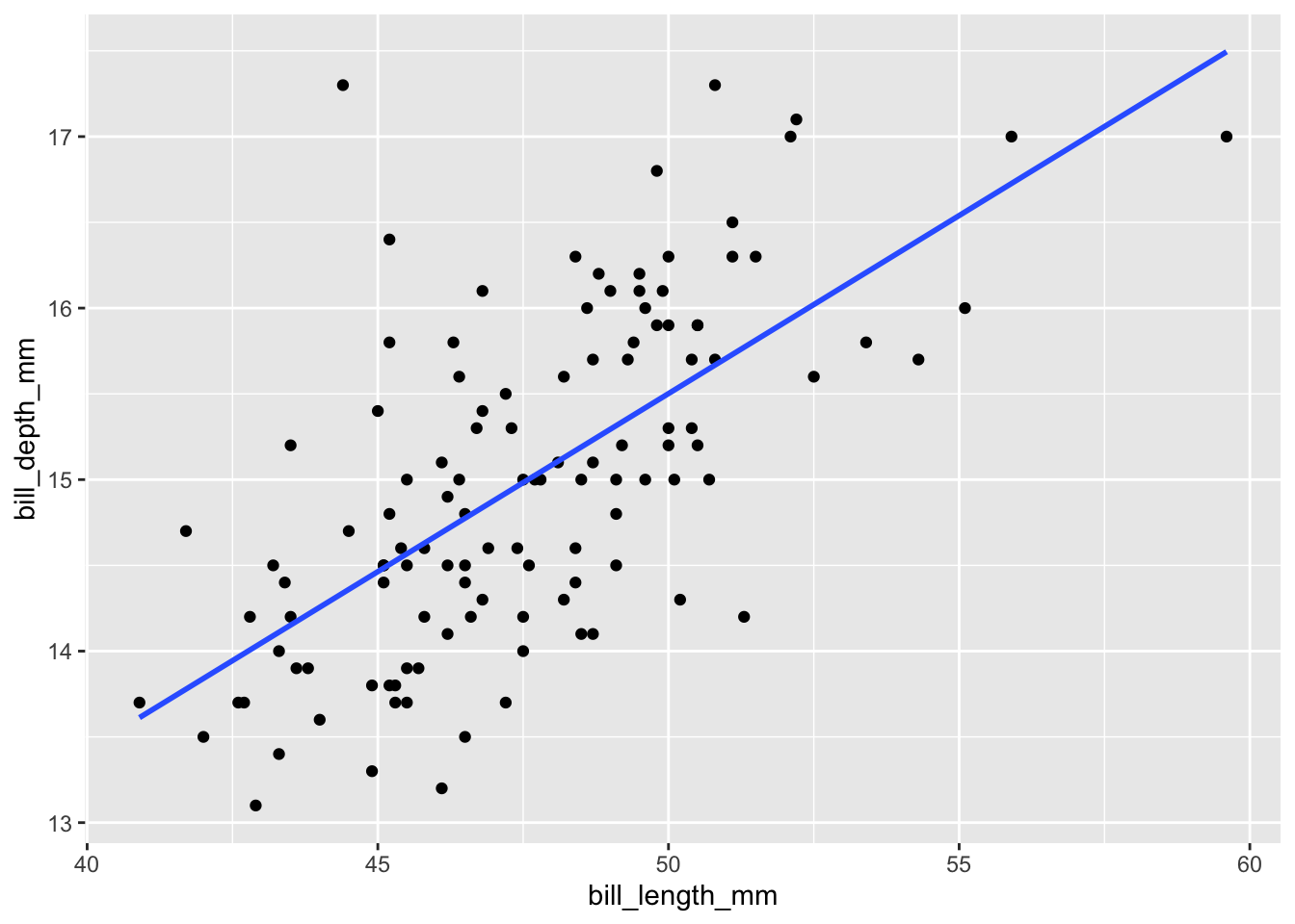
pg_resid <-augment(results)
pg_resid |>
  ggplot(aes(.fitted, .resid))+
  geom_point()+
  geom_hline(yintercept = 0, color= "red") +
  labs(title = "Residual Graph")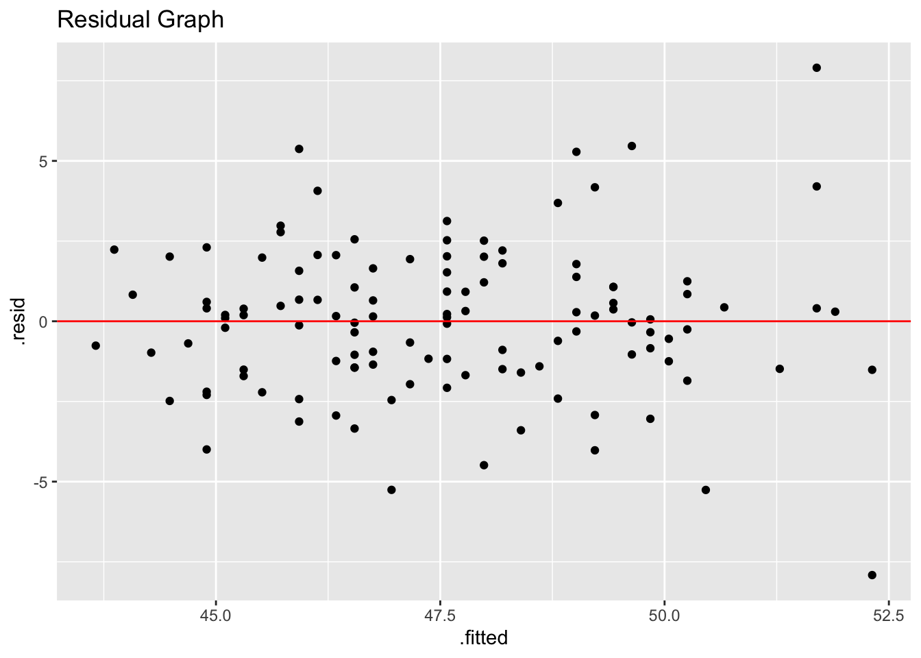
b. Fill in the blanks: The R output displays a linear model for the Gentoo penguins where the response variable is bill_depth_mm and the predictor variable is bill_length_mm.
c. We use the formula for test statistic to get ?.
\(? = \frac{2.020768-0}{0.2185866} \approx 9.244702\)
d. 90% CI
#Lower
2.020768 + qt(0.05, df= 118)* 0.2185866
[1] 1.65838#Upper
2.020768 - qt(0.05, df= 118)* 0.2185866[1] 2.383156e. We would expect an increase in bill depth of 1 mm to yield an increase of about 2.02 mm in body length. If it were possible to have a bill depth of zero we would expect a Gentoo penguin to have a body length of 17.23 .
Problem 6
Test to see if there is a difference between the average flipper length of the Adelie and Chinstrap Penguins. Be sure to discuss all conditions. If you use R, only consider the functions: pt(), qt(), pnorm(), qnorm().
filter(penguins, species %in% c("Adelie", "Chinstrap"))|>
  group_by(species) |>
  summarise(mean = mean(flipper_length_mm),
            sd = sd(flipper_length_mm),
            median = median(flipper_length_mm),
            min = min(flipper_length_mm),
            max = max(flipper_length_mm),
            count = n()) |>
kable(digits = 1)| species | mean | sd | median | min | max | count |
|---|---|---|---|---|---|---|
| Adelie | 190.1 | 6.5 | 190 | 172 | 210 | 146 |
| Chinstrap | 195.8 | 7.1 | 196 | 178 | 212 | 68 |
Problem 7
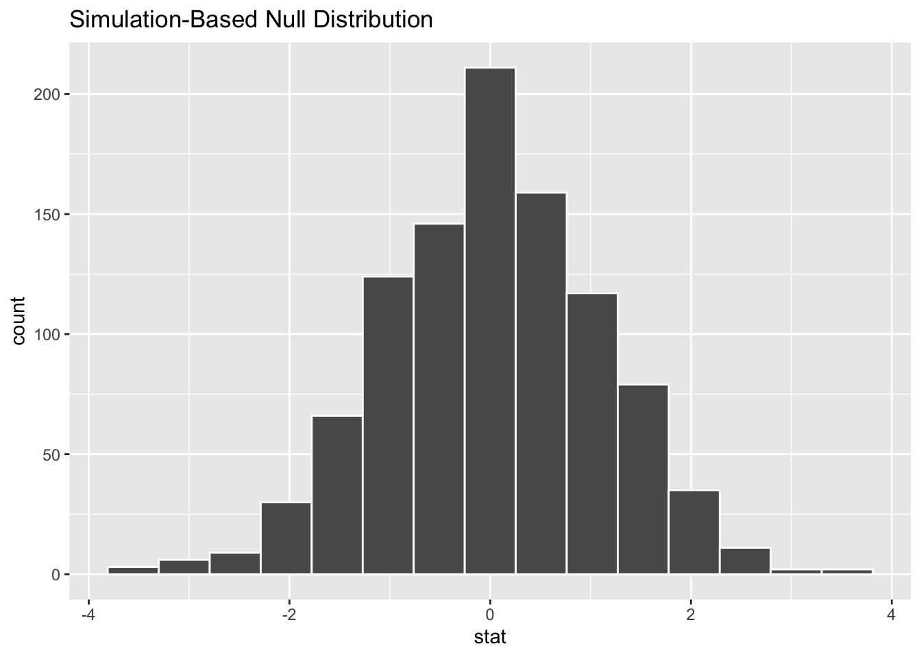
Consider the randomization distribution for the difference in average flipper length of the Adelie and Chinstrap Penguins. Using only information given in the previous problems and the graph below test to see if there is a difference in average flipper between the two selected species at the 1% significance level.
set.seed(62)
penguins |>
  filter(species %in% c("Adelie", "Chinstrap"))|>
  specify(flipper_length_mm ~ species) |>
  hypothesize(null = "independence") |>
  generate(reps = 1000, type = "permute") |>
  calculate(stat = "diff in means", order = c("Adelie", "Chinstrap")) |>
  visualise()