Introduction to R and R Studio
In this class we will use R and RStudio to learn how to analyze real data and come to informed conclusions. To straighten out which is which: R is the name of the programming language itself, and RStudio is a convenient interface for using R.
As the course progresses, you are encouraged to explore beyond what we discuss; a willingness to experiment will make you a much better scientist and researcher. Before we get to that stage, however, you need to build some competence in R. We begin with some of the fundamental building blocks of R and Rstudio: the interface, data types, variables, importing data, and plotting data.
R is widely used by the scientific community as a no-cost alternative to expensive commercial software packages like SPSS and MATLAB. It is both a statistical software analysis system and a programming environment for developing scientific applications. Scientists routinely make available for free R programs they have developed that might be of use to others. Hundreds of packages can be downloaded for all types of scientific computing applications. This handout was written by the help of Dr. Robert Desharnais California State University, Los Angeles and Dr. Kaitlyn Cook.
Getting Started
To get started, you need to download both the R and Rstudio software. Both are available for free and there are versions for Linux, Mac OS X, and Windows. It is suggested that you download R first and then Rstudio. R can be used without RStudio, but RStudio provides a convenient user interface and programming environment for R.
The details for downloading and installing these software packages varies depending on your computer and operating system. You may need permission to install the software on your computer. It is assumed that you already have these programs installed on your system.
The RStudio Interface
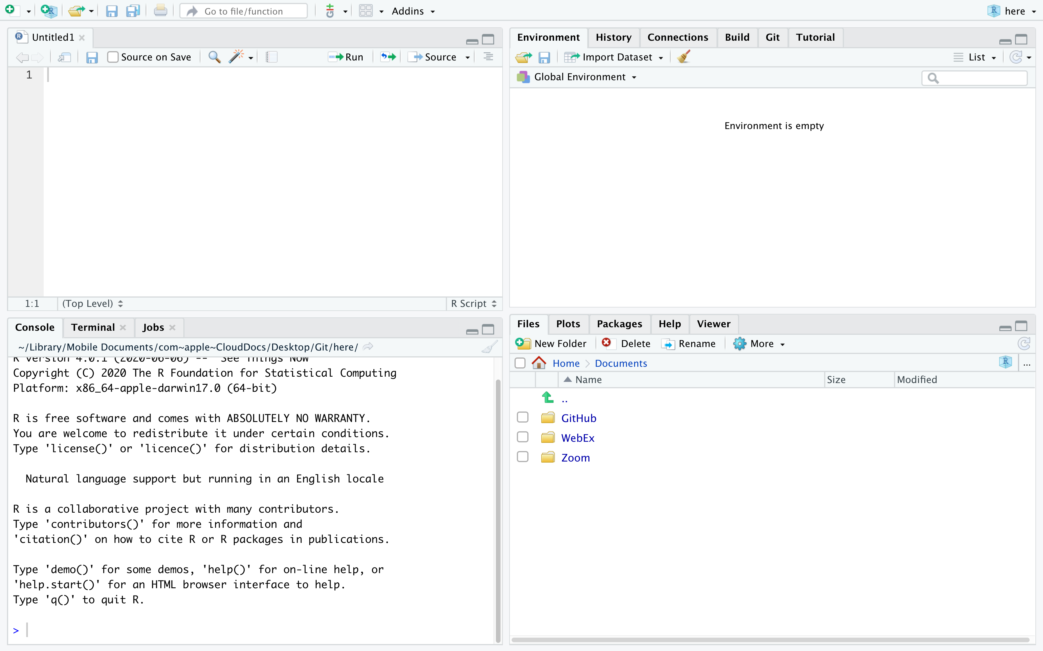
We will begin by looking at the RStudio software interface. The RStudio program is referred to the window, and each section in the interface is a pane.
Launch RStudio. You will see a window that looks like the figure above. The four panes of the window are described as follows:
The pane in the bottom left is the R Command Console, this is where you type R commands for immediate execution.
The pane in the upper left portion of the window is an area for editing R source code for scripts and functions and for viewing R data frame objects. New tabs will be added as new R code files and data objects are opened.
The pane in the upper right portion of the window is an area for browsing the variables in the R workspace environment and the R command line history.
The pane in the lower right portion of the window has several tabs. The Files tab is an area for browsing the files in the current working directory. The Plot tab is for viewing graphics produced using R commands. The Packages tab lists the R packages available. Other packages can be loaded. The Help tab provides access to the R documentation. The Viewer tab is for viewing local web content in the temporary session directory (not files on the web).
Bottom Left Pane
Let’s begin with the Console. This is where you type R commands for immediate execution. Click in the Command Console, “>” symbol is the system prompt. You should see a blinking cursor that tells you the console is the current focus of keyboard input. Type:
1+2[1] 3The result tells you that the line begins with the first (and only) element of the result which is the number 3. You can also execute R’s built-in functions (or functions you add). Type the following command.
exp(pi)[1] 23.14069In R, “pi” is a special constant to represent the number and “exp” is the exponential function. The result tells you that the first (and only) element of the result is the number \(e^{\pi}=\) 23.14069.
Bottom Right Pane
Now let’s look at the Files tab of the notebook at the lower right of the window. Every R session has a working directory where R looks for and saves files. It is a good practice to create a different directory for every project and make that directory the working directory.
Top Right Pane
Next we will look at the R environment, also called the R workspace. This is where you can see the names and other information on the variables that were created during your R session and are available for use in other commands.
In the R console type:
a <- 29.325
b <- log(a)
c <- a/b
Look at the Environment pane. The variables a, b, and c are now part of your R work space. You can reuse those variables as part of other commands.
In the R console type:
v <- c(a, b, c)
v
[1] 29.325000 3.378440 8.680041The variable v is a vector created using the concatenate function c(). (The concatenate should not be confused with the variable c that was created earlier. Functions are always followed by parentheses that contain the function arguments). This function combines its arguments into a vector or list. Look at the Environment panel. The text num [1:3] tells us that the variable v is a vector with elements v[1], v[2], and v[3].
Top Left Pane
Now let’s look at the R viewer notebook. This panel can be used to data which are data frame objects or matrix objects in R.
We will begin by taking advantage of a data frame object that was built into R for demonstration purposes. We will copy it into a data frame object. In the R console, type:
df <- mtcarsLet’s view the data. On the right side of the entry for the df object is a button we can use to view the entries of the data frame. Click on the View Button.
If your look in the notebook area in the upper left portion of the window, you can see a spreadsheet-like view of the data. This is for viewing only; you cannot edit the data. Use the scroll bars to view the data entries.
You can also list the data in the console by typing the name of the data fame object:
df mpg cyl disp hp drat wt qsec vs am gear carb
Mazda RX4 21.0 6 160.0 110 3.90 2.620 16.46 0 1 4 4
Mazda RX4 Wag 21.0 6 160.0 110 3.90 2.875 17.02 0 1 4 4
Datsun 710 22.8 4 108.0 93 3.85 2.320 18.61 1 1 4 1
Hornet 4 Drive 21.4 6 258.0 110 3.08 3.215 19.44 1 0 3 1
Hornet Sportabout 18.7 8 360.0 175 3.15 3.440 17.02 0 0 3 2
Valiant 18.1 6 225.0 105 2.76 3.460 20.22 1 0 3 1
Duster 360 14.3 8 360.0 245 3.21 3.570 15.84 0 0 3 4
Merc 240D 24.4 4 146.7 62 3.69 3.190 20.00 1 0 4 2
Merc 230 22.8 4 140.8 95 3.92 3.150 22.90 1 0 4 2
Merc 280 19.2 6 167.6 123 3.92 3.440 18.30 1 0 4 4
Merc 280C 17.8 6 167.6 123 3.92 3.440 18.90 1 0 4 4
Merc 450SE 16.4 8 275.8 180 3.07 4.070 17.40 0 0 3 3
Merc 450SL 17.3 8 275.8 180 3.07 3.730 17.60 0 0 3 3
Merc 450SLC 15.2 8 275.8 180 3.07 3.780 18.00 0 0 3 3
Cadillac Fleetwood 10.4 8 472.0 205 2.93 5.250 17.98 0 0 3 4
Lincoln Continental 10.4 8 460.0 215 3.00 5.424 17.82 0 0 3 4
Chrysler Imperial 14.7 8 440.0 230 3.23 5.345 17.42 0 0 3 4
Fiat 128 32.4 4 78.7 66 4.08 2.200 19.47 1 1 4 1
Honda Civic 30.4 4 75.7 52 4.93 1.615 18.52 1 1 4 2
Toyota Corolla 33.9 4 71.1 65 4.22 1.835 19.90 1 1 4 1
Toyota Corona 21.5 4 120.1 97 3.70 2.465 20.01 1 0 3 1
Dodge Challenger 15.5 8 318.0 150 2.76 3.520 16.87 0 0 3 2
AMC Javelin 15.2 8 304.0 150 3.15 3.435 17.30 0 0 3 2
Camaro Z28 13.3 8 350.0 245 3.73 3.840 15.41 0 0 3 4
Pontiac Firebird 19.2 8 400.0 175 3.08 3.845 17.05 0 0 3 2
Fiat X1-9 27.3 4 79.0 66 4.08 1.935 18.90 1 1 4 1
Porsche 914-2 26.0 4 120.3 91 4.43 2.140 16.70 0 1 5 2
Lotus Europa 30.4 4 95.1 113 3.77 1.513 16.90 1 1 5 2
Ford Pantera L 15.8 8 351.0 264 4.22 3.170 14.50 0 1 5 4
Ferrari Dino 19.7 6 145.0 175 3.62 2.770 15.50 0 1 5 6
Maserati Bora 15.0 8 301.0 335 3.54 3.570 14.60 0 1 5 8
Volvo 142E 21.4 4 121.0 109 4.11 2.780 18.60 1 1 4 2The columns are labeled with the names of the variables and the rows are labeled with the names of each car. Each row represents the data values for one car; that is, each row is one observation.
Recommended Settings
R has many features and customizable options. Below are a few recommended settings. You only need to complete these steps once. Click on Tools > Global Options and change the following:
Under General > Basic, uncheck ‘Restore .RData into workspace at startup’
Under R Markdown > Visual, uncheck ‘Use visual editor by default for new documents’
Under Appearance, pick any theme you like
I also strongly recommend that you create a new project for SDS 220: a place to store all of your files, assignments, and datasets for this class.
Next, we will install a few extra features using a library. Run the following commands in your console. These only need to be ran once.
install.packages("tidyverse")
install.packages("tinytex")
tinytex::install_tinytex()
Object Types
In R, data can be stored in more complex structures. The most critical object types we will use are vectors, and data frames. Most statistical analyses are performed using data stored in data frames.
Vectors
Vectors are one of the fundamental building blocks for data storage in R. We can create them by concatenating a series of data elements using the function c(). For example, suppose this vector contains the number of siblings for the students sitting next to you.
c(1, 3, 0, 2, 0)[1] 1 3 0 2 0We can store our created vector in the computer to a name using the assignment operator <-.
siblings <- c(1, 3, 0, 2, 0)The utility of vectors isn’t limited to numeric data only. We can use vectors to store many different types of data. For example, we can store the reported houses for the students we sit next to.
house <- c("Tyler", "Capen", "Hubbard", "Hubbard", "Cutter")There are three main classes of vectors in R, organized according to their broad attributes and behaviors:
- Numeric: composed of (discrete and continuous) numbers
- Character: composed of text
- Factor: composed of text with a finite number of possible values (‘levels’) and the possibility of a sense of order or ranking to those levels
We use vectors to store information about variables. So the taxonomy for types of variables immediately translates into a taxonomy for classes of vectors in R. We can use the class() function to see how the type of vector the computer has stored.
class(siblings)[1] "numeric"class(house)[1] "character"Factor vectors are typically not created in R by default. To create an explicit factor vector we must use the factor function.
house.fac <- factor(house)
house.fac
[1] Tyler Capen Hubbard Hubbard Cutter
Levels: Capen Cutter Hubbard Tylerclass(house.fac)[1] "factor"Now we have the objects house and house.fac. The first is a character vector, and the second is a factor vector.
Data Frames
We can combine multiple vectors of the same length into a 2-D structure called a dataframe, which is the main form in which we store and work with data in R:
class.data <- data.frame(siblings, house)
class.data
siblings house
1 1 Tyler
2 3 Capen
3 0 Hubbard
4 2 Hubbard
5 0 CutterWe call these data tidy if they map neatly back to our terminology from before:
Each row is an observational unit
Each column is a variable
We can still access the individual data vectors using the $ operator:
class.data$siblings[1] 1 3 0 2 0Naming Conventions
R has rules when it comes to naming objects. An object may start with a letter or a ., and the remaining characters may consist of letters, digits, . or _. There are also special types of objects that have already established names in R. For example, NULL, TRUE, FALSE, if, and function should not be used as a new object name. To see a list of these reserved object names type ?Reserved in to your console.
Core Features
Arithmetic Operators
An operator is a symbol that tells the compiler to preform a specific task. R was designed for statistical applications and as a necessity it needs to preform mathematical operations efficiently and effectively. The first operators we discuss are a few of the basic arithmetic operations. These are operations similar to that of a calculator.
# Addition
2 + 3
[1] 5# Subtraction
2 - 3[1] -1# Multiplication
2*3[1] 6# Division
2/3[1] 0.6666667# Exponent
2^3[1] 8Assignment Operators
Assignment operators are used to assign values to a new object. There are many types of assignment operators, and they operate slightly differently. The two most common assignment operators are = and <-. With these operators the value to the left of the operator is the name of the new object and the value on the right is what the object is now equal to.
x = 5
x
[1] 5x <- 5
x[1] 5The majority of the time we can use these two assignment operators above interchangeably, there are some exceptions though. There are several other assignment operators which are uncommon and should only be used by advanced users, ->, <<-, and ->>.
When we create new objects it is called binding. Consider the code below.
v <- c(6, 2, 5)In this line of code the object c(6, 2 ,5) is binded to the name v. That is, v acts as a reference (or a placeholder) for the object c(6, 2, 5). Everywhere we see the object v we should mentally replace it with this vector.
Basic Calculations
There are many functions in R that work similarly to how we would see in excel, or in a calculator. Most of these calculator-like functions take in a vector as input.
abs(): Takes in a vector, and returns the absolute value of each element in the vector.sum(): Takes in a vector, and returns the sum of all element in the vector.prod(): Takes in a vector, and returns the product of all elements in the vector.exp(): Takes in a vector, and returns \(e\) to the power of each element in that vector (i.e. \(e^x\))log(): Takes in a vector, and returns the NATURAL LOG of each element in the vector.log10(): Takes in a vector, and returns the log (base ten) of each element in the vector.mean(): Takes in a vector, and returns the mean of the values in the vector.median(): Takes in a vector, and returns the median of the values in the vector.var(): Takes in a vector, and returns the variance of the values in the vector.sqrt(): If you give it a vector, it returns the square root of each element in the vector. If you give it a single number, it returns the square root of the number.sd(): Takes in a vector, and returns the standard deviation of the values in the vector.range(): Takes in a vector, and returns the minimum AND maximum of the values in the vector.
Notice also that these functions take a single vector as input. Consider the following two examples.
# Calculate the mean
mean(c(1, 2, 3))
[1] 2# Calculate the square root
sqrt(v)[1] 2.449490 1.414214 2.236068Document Types
We have two main types of documents that we will use in this class.
R Scripts:
.Rfiles that function a bit like recipes, in that they allow us to write and save the instructions (code) for processing data and running analysesQuarto Documents:
.qmdfiles that allow us to integrate our R code and data visualizations alongside written text
The Quarto documents are created by
File -> New File -> Quarto Document…
In the popup create a title and select “pdf”
We will Quarto files to create our homework!
Comments
Often times we will want to add a comment to our script document so we can remember special aspects later, and make the code easier to read and modify in the future. To add a comment start the comment with a
#symbol. This will make the remaining characters in a line a comment and R will not try to compile these lines. Go to the script document and type the following. Highlight what you have typed and press “Run”.